Bayesian Inference with Markov Chain Monte Carlo in Clojure
12 Mar 2014I've been working through the book Probabilistic Programming and Bayesian Methods for Hackers (ProbHack) by Cam Davidson-Pilon. This online book is an introduction to bayesian methods and probabilistic programming for programmers. Its main focus is Bayesian Inference with Markov Chain Monte Carlo (BI-MCMC). The ProbHack book uses Python and the PyMC library. For my own understanding of the inner-workings of BI-MCMC I ported the code to Clojure in the bi-mcmc (bi-mcmc) project on github.
BI-MCMC Algorithm
Rather than requiring intricate mathematical knowledge to be able to derive a numerical solution, BI-MCMC uses an algorithm to iteratively arrive at the solution. It even turns out that the iterative solution is needed for cases where deriving the solution is impossible. I don't know whether the fourth order partial derivative of co-prime free variables are convex and therefore have a closed form solution for the global optima. I do know how to code a loop. BI-MCMC luckily requires more knowledge of the latter rather than the former.
Bayesian Inference refers to a Bayesian model where probability distributions produce data. The inference part is to find the parameters of the probability distributions. Usually the answers for the parameters are probability distributions themselves. The answers will not be single numbers, but rather distributions that show certainty (or uncertainty) and deviations for the answers.
The Markov Chain Monte Carlo (MCMC) part is the iterative algorithm that can find the probability distributions for the parameters of the Bayesian model using simulation and sampling. A truly naive iterative algorithm would try every possible combination of the possible values for the parameters. Through combinatorial explosion this is unfeasible for most interesting models. MCMC only considers part of the solution space.
The main example in the ProbHack book is an "sms/texts received per
day" received example:
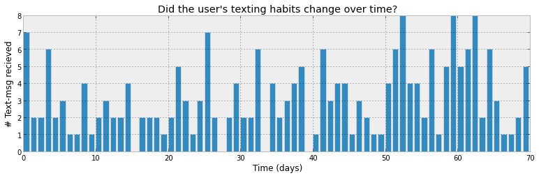 Image from: ProbHack
The idea is that the number of texts per day is defined by a Bayesian model. The question is: what are the parameters of that Bayesian model? BI-MCMC can answer that question by giving a probability distribution for the parameters. Note that the Bayesian model will be defined in terms of probability distributions and that the parameters of those distributions are probability distributions themselves.
The model for the texts example looks like this:
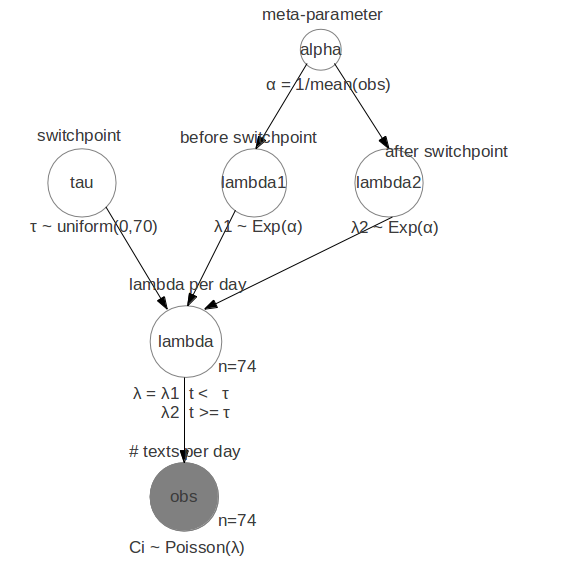 For all days before tau the expected number of text messages is a
Poisson distribution with parameter lambda1. For all days after tau
the expected number of text messages is a Poisson distribution with
parameter lambda2. The question we want answered is when day tau is
and what the likely values for lambda1 and 2 are. In the ProbHack book
the real world reason for the detected change in number of texts per
day is given.
For all days before tau the expected number of text messages is a
Poisson distribution with parameter lambda1. For all days after tau
the expected number of text messages is a Poisson distribution with
parameter lambda2. The question we want answered is when day tau is
and what the likely values for lambda1 and 2 are. In the ProbHack book
the real world reason for the detected change in number of texts per
day is given.
The way BI-MCMC works is basically trying a lot of different combinations for the values of tau, lambda1 and lambda2. Each of those combinations is a sample. At the end of the simulation all the values for the parameters are the probability distribution for the parameters. These can be visualized with histograms for example. This works because the samples are generated in such a way that there are more samples created with more likely values for each of the parameters.
For example consider this sample from a simulation (sample 50178 out of 100000):
{:observation {:logp -481.660, :self-logp -481.660,
               :value [.. fixed data ..]},
 :lambda {:logp -481.660, :self-logp 0.0,
          :value [17.740 .. until tau ...
                  24.210 .. after tau ..]},
 :lambda1 {:step-sd 118.049, :step-scale 0.0196,
           :logp -485.542, :log-ratio 0.222,
           :self-logp -3.881, :prev-logp -485.764,
           :proposed 17.740, :prev-value 16.763,
           :value 17.740,
           :why :accepted,
           :accepted-by-flip 5464,
           :accepted 11012,
           :rejected 39166},
 :lambda2 {:step-sd 17.950, :step-scale 0.185,
           :logp -487.166, :log-ratio -0.133,
           :self-logp -4.209, :prev-logp -487.032,
           :proposed 24.210, :prev-value 21.496,
           :value 24.210,
           :why :accepted-by-flip,
           :accepted-by-flip 5311,
           :accepted 10748,
           :rejected 39430},
 :tau {:step-sd 42.0, :step-scale 0.070,
       :logp -484.999, :log-ratio -22.394,
       :self-logp -4.304, :prev-logp -484.999,
       :proposed 47, :prev-value 45,
       :value 45,
       :why :rejected,
       :accepted-by-flip 5877,
       :accepted 10348,
       :rejected 39830}}
All the variables in the sample have the probability of their value, using the current values of the other variables in the sample, under the :logp and :logp-self keys. The :logp is the most important value, because it show the likeliness of the value for the variable given all the variables it is dependent on. The :logp value is used to decide whether a sample is accepted or rejected.
The data for :observation is always the same as it is given. Only its :logp and :logp-self values change per sample when the other variables change and make it likelier or unlikelier to have generated this data. The value for :lambda is calculated again for every sample based on the changing variables. The :lambda1, :lambda2 and :tau variables are the interesting ones, because they are stochastic variables. In every sample the values for :lambda1, :lambda2 and :tau are generated based on their values in the previous sample (hence the Markov Chain part in the BI-MCMC name). When the new proposed value has a higher probability (:logp) of creating the observed data, then this becomes the new value for the variable in the sample. When there is a lower probability then the value is accepted by a coin-flip, proportional to how unlikelier the new value is. This sample includes all three cases of a proposed value being :accepted, :accepted-by-flip and :rejected. This procedure creates samples where the values for the variables form the probability distributions for the variables. The particulars about this random walk procedure are discussed in the ProbHack book.
How much a value of a stochastic variable is changed each sample is drawn from a normal distribution with the :step-sd and :step-scale parameters. Together these form the standard deviation. With a bit of meta-learning based on the last 1000 samples the :step-scale is adjusted based on the number of :accepted and :rejected proposals. This makes sure that only reasonable values for the variables are proposed.
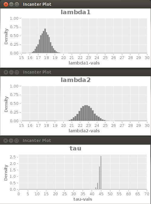
Probability distributions for the variables based on the BI-MCMC samples.
Clojure code vs. Python code
The code used in the ProbHack book uses the Python PyMC library. In the PyMC library the Bayesian model is modeled as a mutable object graph, where the objects are stochastic or deterministic variables. For each sample the fields of the objects are changed and possible reverted upon rejection. The Clojure code uses a more functional approach. The structure of the Bayesian model is a data structure while the values are only available as samples. With this structure running the MCMC algorithm is indeed just a Clojure loop invoking a function on data for each sample.
Of course the bi-mcmc project is far from complete and I have no plans to develop it further. In particular it is quite slow for variables with many values. This is case for the clusters example, where a single variable has 1000 observed values. There is a possibility for a speed-up here by using transients or even a mutable datastructure, because the data won't be changed once it is shared.
The MCMC algorithm has a natural multi-threaded extension. Samples from different random walks can be combined to create the probability distributions for the parameters. It should be a straight forward extension on top of the functional design to run multiple runs concurrently.
For the graphs and probabilities the incanter library is used. The design of the probability package turned out to be a bad fit for this project. In bi-mcmc the probability density function of a distribution is needed most often. However the parameters of the distributions change per sample. What I needed are functions that give the likelihood given some parameters and a value. Instead the incanter library builds a distribution with a constructor, which has a pdf function with a value as argument. This is due to the underlying Java library that incanter wraps. In order to get the density of a value for a different distribution it actually needs to call a function called .setState! For this project wrapping the static methods from SSJ would have been better.